Getting started
On this page you learn how to run a solver from one of our starter kits against a training simulation of the hotstorage track. The procedure for participating in the rolling mill track is the same and the starter kits contain code for that as well.
We offer starter kits in four different languages. The implementations provided in these kits are equal. Each contains a very simple rule-based approach and a heuristic based on depth-first search. These should demonstrate the interaction between the solver and the simulation. The following four kits are available:
If you would like to contribute a starter kit in another language, please send us a pull request. To continue with the tutorial you must clone the repository to your computer.
The kits are subfolders in that repository, e.g. starterkits/csharp for the C# kit. For the rest of the tutorial we assume that you have built the solver of your choice successfully.
Build the starter kit that you want to use by following the build instructions in the respective Readme.md file.
Set up a new training simulation
The Experiments page contains all the simulation runs and associated results that you have created so far. The page is divided into training and scoring experiments. In this tutorial we will create a training experiment and run the solver against it. Scoring experiments are special and will be covered on the Documentation page. To proceed with this tutorial you have to create a user account on this website and have to be logged in!
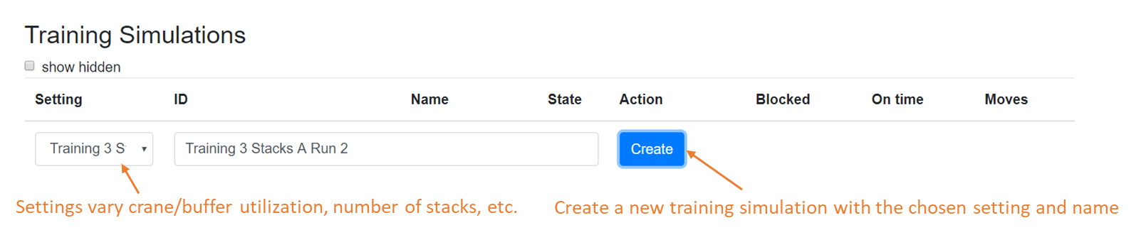
Each setting represents a different configuration of the simulation. In one setting the utilization may be higher, for instance new blocks may arrive faster and/or stay longer in the system. This creates different challenges for your solver. We will not disclose the exact parameters of these settings, but statistics and KPIs will be collected that you can use to adapt the solver.
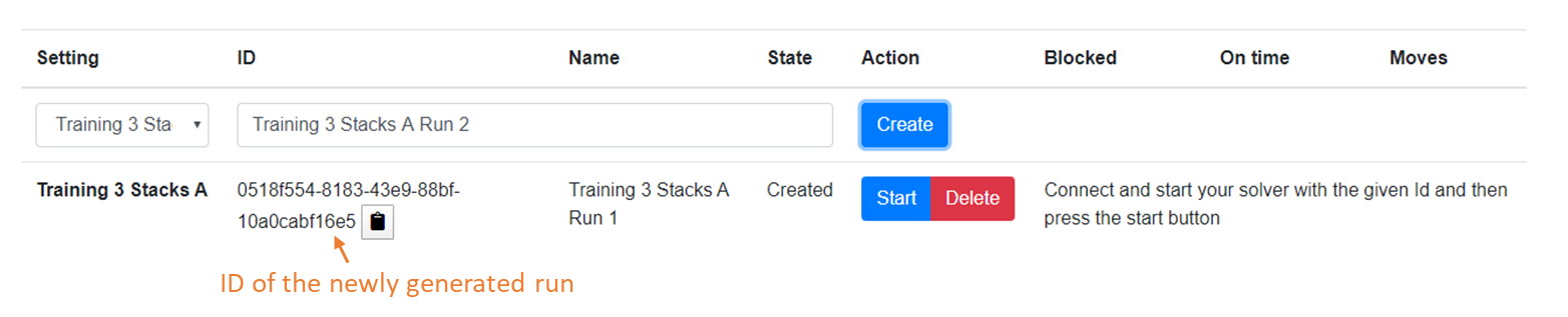
Now it is time to start your solver. Connect it with the simulation and then start the simulation run on this website. If you start the run before you start your solver you might miss some of the action! On the top of the Experiments page you see an URI for connecting with the simulation. The solver in the starter kit needs to know this URI, the simulation ID and wether it is a hotstorage (HS) simluation or a rollingmill (RM) simulation.
You will see that this was successful as the solver outputs
ModelBased
Connected
Start the training simulation and visualize the results
Training runs are for testing your implementation during the development of your solver. You can do as many training runs as you like to improve your solver. However, you may run only four simulations simultaneously. You first have to complete some runs to start more. These training runs are not used to determine the ranking in the competition!
Now the simulation is running and the solver is receiving updates from the simulation state, so called world updates. The solver reacts to these updates by sending crane schedules to the respective URI. A crane schedule contains a list of moves. The simulation will check if a certain move is invalid, in which case it will skip it and continue with the next move in the schedule.
The starter kit will not really produce very meaningful results out of the box. It will be your challenge to develop a meaningful solver, potentially by expanding what we have in the starter kit.
View the performance of the solver
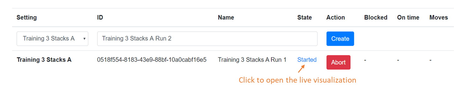
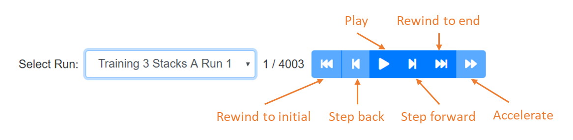
On the Visualization page you can select the simulation run that you want to watch in the dropdown list. For running simulations you have the option to either replay the history so far, or view its live state.
When you select a simulation run you see its initial state of the world. You can click on the play button to view it in realtime, but you may accelerate using the forward button. You can also step through the simulation and fast-forward to the end or fast-rewind to the beginning.
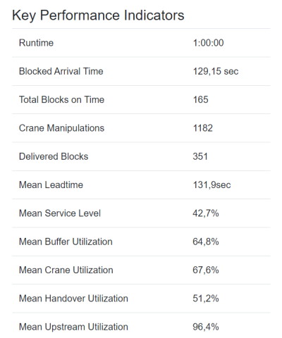
Below the world visualization you find the KPIs that quantify the so called offline performance of your policy. The top three, after Runtime, are counted for the ranking of your policy. The others are for your analysis.